Best time to post on HackerNews
July 2, 2021
Let’s determine what the best time to post on HackerNews using statistical analysis and machine learning is.
Mining HackerNews
Hackernews (HN) has become one of the primary resources to share and discuss tech community news. On average, we share 133 posts daily, leaving 6 comments on each one. If you read this article, you likely post on HN too. You may also wonder the best time to post and what topics interest the HN audience most. If so, that’s good news. In this article, we will use statistical analysis to find the best time interval to get upvotes. After that, we will seek historical data for common topics that HN users enjoy.
If you want to play with the code provided for this repository, you can find the complete analysis at this GitHub repo. I will also provide links to Google Colab for Jupyter notebooks throughout the post.
How fast do you get upvotes?
The best time to post may vary according to your goals. We will use upvote count as the primary metric of success. To find the best time intervals, I’ve collected a couple of months’ worth of data that contains post and comment updates for every few minutes.
First, let’s see how fast posts accumulate 95% of upvotes. If you look at random plots of score cumulative sum over time, you will get something like this:
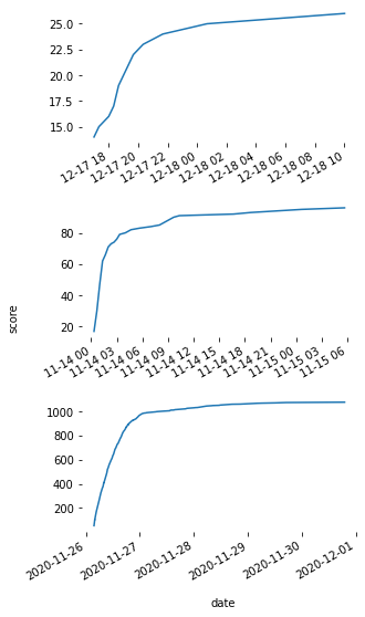
Looks like a logarithmic function, right? This means that we can fit logarithmic function for historical data of each post to get a smooth estimate of a score accumulation curve: \(f(x) = a * log(x) + b\). We can use numpy to find a and b parameters for each post, resulting in the closest logarithmic approximation we can get:

If you then measure when returns start to get less than 5% after each time interval, you will get a time during which each post will get 95% upvotes. In the case of this dataset, we can see that, in general, 2 hours is enough.
Finding the best time to post on HN
To find the best hours to post on HackerNews, we will multi-stage analysis. At first, we will look at empirical statistics that we can collect from the dataset: mean, median, and standard deviation per each stratum (slice) of data of interest. First, we will look at score statistics per weekdays:
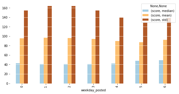
Here, we can see that Mondays and weekends are arguably the best time to post. Then, let’s look at hours:

This plot suggests that 4–5 AM is the best time to post, along with the 21–23 hour interval.
To confirm ideas that we got from the exploratory data analysis, we will use regression analysis of the following equation:
\[score = \beta_0 + \beta_{1..24}C( hour)\] \[score = \beta_0 + \beta_{1..7}C( weekday)\]where C means one-hot encoding. We will have a separate binary variable and a coefficient for each hour.
You may wonder why we use more advanced techniques such as gradient boosting, neural networks, and a plethora of available algorithms? The problem is that most of the machine learning algorithms seek to solve prediction problems. What we want instead is to perform statistical inference. When you try to solve a prediction problem, your goal is to optimize for likelihood, mean squared error, or another metric of choice. The primary objective is to get a better model. When you solve a statistical inference problem, you seek statistically useful answers based on your data. In this case, you do not care for model accuracy, but instead, try to infer answers to your questions using statistical models. Statistical inference is the problem we are trying to solve. Thus we go with it. The important question is whether we should use a standard Gaussian regression. Let’s look at the score distribution plot:
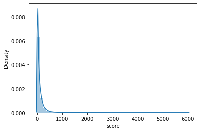
Doesn’t look like a gaussian, right? The plot suggests a Poisson distribution. We are using count data, so this makes sense. If you run some statistical tests or perform a simple dispersion test (for Poisson, mean should equal variance). This means that Poisson regression is not the best model to use in our case. The second alternative in case of overdispersion is Negative Binomial distribution, which we will actually use. We fit our models, sort coefficients, and get the following results:
We can also look at the mixed GLM model class, which will allow us to account for variance effects between different weekdays. For this class of models, we will get a slightly different ranking:
| Hour posted | coef | std err | z | P>z | [0.025 | 0.975] |
|---|---|---|---|---|---|---|
| 8 | 4.6401 | 0.009 | 518.146 | 0.000 | 4.623 | 4.658 |
| 9 | 4.6309 | 0.009 | 531.683 | 0.000 | 4.614 | 4.648 |
| 11 | 4.6300 | 0.008 | 572.639 | 0.000 | 4.614 | 4.646 |
| 10 | 4.6217 | 0.008 | 567.044 | 0.000 | 4.606 | 4.638 |
| 7 | 4.6167 | 0.009 | 494.065 | 0.000 | 4.598 | 4.635 |
| 12 | 4.5831 | 0.008 | 563.120 | 0.000 | 4.567 | 4.599 |
| 6 | 4.5789 | 0.010 | 455.735 | 0.000 | 4.559 | 4.599 |
| 5 | 4.5617 | 0.011 | 415.651 | 0.000 | 4.540 | 4.583 |
| 4 | 4.5440 | 0.012 | 383.083 | 0.000 | 4.521 | 4.567 |
| 1 | 4.5318 | 0.013 | 357.098 | 0.000 | 4.507 | 4.557 |
| 3 | 4.5298 | 0.012 | 371.023 | 0.000 | 4.506 | 4.554 |
| 13 | 4.5257 | 0.008 | 548.687 | 0.000 | 4.510 | 4.542 |
| 2 | 4.5156 | 0.013 | 360.607 | 0.000 | 4.491 | 4.540 |
| 21 | 4.4920 | 0.012 | 372.377 | 0.000 | 4.468 | 4.516 |
| 22 | 4.4889 | 0.012 | 365.875 | 0.000 | 4.465 | 4.513 |
| 14 | 4.4876 | 0.009 | 527.204 | 0.000 | 4.471 | 4.504 |
| 23 | 4.4780 | 0.012 | 358.526 | 0.000 | 4.454 | 4.502 |
| 0 | 4.4629 | 0.013 | 352.764 | 0.000 | 4.438 | 4.488 |
| 16 | 4.4575 | 0.009 | 485.264 | 0.000 | 4.439 | 4.475 |
| 15 | 4.4515 | 0.009 | 508.004 | 0.000 | 4.434 | 4.469 |
| 17 | 4.4495 | 0.010 | 450.631 | 0.000 | 4.430 | 4.469 |
| 18 | 4.4399 | 0.010 | 423.904 | 0.000 | 4.419 | 4.460 |
| 20 | 4.4386 | 0.012 | 383.671 | 0.000 | 4.416 | 4.461 |
| 19 | 4.4361 | 0.011 | 397.220 | 0.000 | 4.414 | 4.458 |
Another interesting question to answer is on which day to post? For this, we can fit a regression model on weekdays and get the following ranking:
| Weekday number | coef | std err | z | P>z | [0.025 | 0.975] |
|---|---|---|---|---|---|---|
| 1 | 4.5750 | 0.005 | 891.534 | 0.000 | 4.565 | 4.585 |
| 2 | 4.5684 | 0.005 | 888.391 | 0.000 | 4.558 | 4.579 |
| 0 | 4.5578 | 0.005 | 877.741 | 0.000 | 4.548 | 4.568 |
| 3 | 4.5432 | 0.005 | 879.076 | 0.000 | 4.533 | 4.553 |
| 6 | 4.5238 | 0.006 | 770.599 | 0.000 | 4.512 | 4.535 |
| 4 | 4.4970 | 0.005 | 839.649 | 0.000 | 4.487 | 4.508 |
| 5 | 4.4706 | 0.006 | 739.867 | 0.000 | 4.459 | 4.482 |
Combined insights from visual analysis, GLM, and Mixed Effects GLM suggest that the best time to post would be on Sunday–Tuesday between 10 and 11 AM EST. Having figured this out, let’s move on to topic analysis.
UPDATE
Since I first wrote a draft of this post, I have used this dataset in another analysis. If you want to see a deeper Bayesian exploration of this dataset please refer to this report.
In general, this report agrees with the analysis above. However, it gives us wider timeframe in terms of best posting hours:

Extracting topics from HN
Let’s find out what topics do the HackerNnews community talks about? To find out, we will open our topic modeling toolbox and extract topics from post titles. You can find several approaches ranging from classic LDA-based models and ending with deep learning methods in the notebook. The technique that showed the best results is called Top2Vec. In short, this approach does the following:
- Take sentence/word embeddings from pertained BERT encoder
- Decrease dimensionality of embeddings
- Cluster them using hierarchical clusters
- Take cluster centroids as topic vectors
- N closest words for each centroid would then be topic keywords
This pipeline is assembled in a ready-to-use package, which you can find here. I discovered that Top2Vec can overfit grammatical structures and cluster them together as a topic, which you should consider when using this method.
If we fit Top2Vec for 15 topics, we can get a feel of what the HN community likes to talk about:
- “How to” posts
- New product or feature announcements, advanced tutorials
- 2-3 word titles. Mainly tech releases
- Negative news about large tech companies, lawsuits
- Politics
- Salary, job change, layoffs
- Programming language & coding tutorials
- Science news
- Security
- CEO/billionaire news
- Tech history
- COVID
- Software engineers hard&soft skills, learning materials
- How tech&AI influences our lives?
- Apple news
Those results can be informative by themselves. However, the original idea of using topic modeling was to discover hidden topics, where posts have more probability of receiving a high score. To analyze this, I have used a technique called Bayesian regression. The model I have analyzed used 50 topics instead of 15, because this setup was more stable in terms of topic distribution variance for different model fits. The results remind us how important it is to look at uncertainty around point estimates. Looking at point estimates alone, we could give a conclusion that there are best and worst topics, but in reality, data shows the opposite.
Analysis showed that there are no best topics, and distributions for each topic found are really wide, as you can see from this plot:
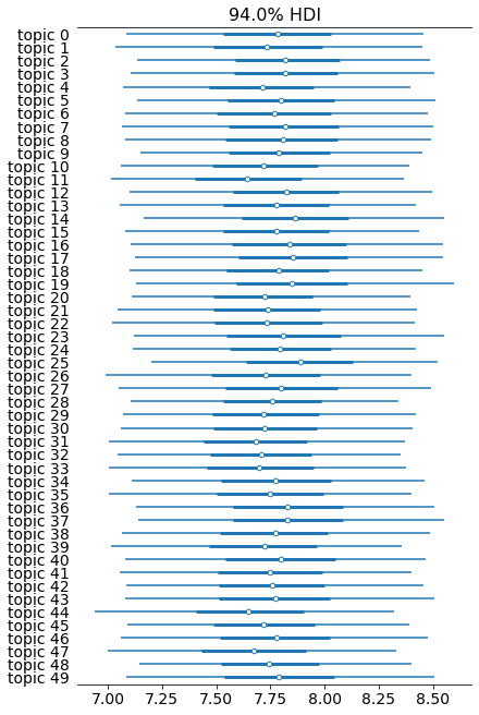
For this analysis, I built a model with 50 topics, which might not be as interpretable, but could find niche topics that deviate from the mean. Each bar represents score distribution among each topic the model found, center point in each row is the average parameter value, and the bold line is a 94% Highest Density Interval. As you can see, there are no best topics. However, there are a couple of topics that look noticeably below average. Let’s look at some example titles from a topic with the lowest average posterior mean:
- Topic 11. Keywords: favorite, favorite, survey, thoughts, which, poll, whats, recommendations, who, predict, predictions, ama, best, longest, examples, alternatives.
We can conclude that this topic primarily consists of questions and discussions by looking at random post samples.
- What do you wear to work?
- What service or product would you be customer 1 for?
- Which tool do you use to configure your DNS entries?
Nonetheless, this does not mean that you absolutely shouldn’t use this topic for the highest scores. Note how wide the distribution for topic 11 is.
I have performed experiments with various topic sizes ranging from 10 to 200, using both flat and hierarchical bayesian models, and the picture stays relatively the same. If you are interested in how this analysis was done, refer to the code for this section.
Conclusion
Much more is still left to be done to make a proper Bayesian analysis of the data: posterior and prior predictive checks, evaluating models using PSIS LOO CV, prior sensitivity analysis. The list goes on and on. However, I feel like moving on to another project 🙂 Ping me if you wish to see more extensive research on this data.
The primary conclusion from this analysis is that the HackerNews community clicks the upvote button most actively between Sunday–Tuesday from 10 to 11 AM EST (or to 3 PM EST according to the second Bayesian analysis), mostly independently of the post topic.